Processing of Regularly-Sampled Spectral Line Maps

Spectral line maps acquired using position-switching or beam-switching result in a grid of data that is uniformly-sampled in angle on the sky. This allows for a streamlined data reduction process. In this example, we will process a 20'x20' map of the 492 GHz fine structure line of atomic carbon in the rho Ophiuchus molecular cloud, taken in position-switching mode with the AST/RO telescope at the South Pole. The reduction of position-switched HHT data is identical.
First, all spectra must have their baselines, and any other instrumental artifacts, removed. This can be done routinely using a loop function in CLASS. We will first load the data file, filtering just the applicable observations, setting an output file, and defining the window in which the spectral line lies (and not to be included in the baseline calculation):
    LAS> find
    I-FIND 1691 observations found
    LAS> set win 0 6
    LAS> file out reduced.dat new
    LAS> for i 1 to found
      LAS: get next
      LAS: base 1
      LAS: plot
      LAS: write
      LAS: next
At this point, all 1691 spectra found by find will be
operated upon by the loop. In this example, we load the next
spectrum, remove a linear baseline, plot the result to the screen,
write the data to the output file reduced.dat, and then
increment the observation number and repeat the process for the next
spectrum. The loop will terminate when the last spectrum is
processed.
Now we can load the processed data file in:
    LAS> file in reduced.dat
I-INPUT,  reduced.dat successfully opened
    LAS> find
    I-FIND 1691 observations found
We can get a first look at the data using the map command.
Map will attempt to plot all 1691 spectra on the screen
simultaneously, with each spectrum at the appropriate offset. First,
the X and Y axis scales must be fixed, the plotting window cleared,
and then map can be invoked:
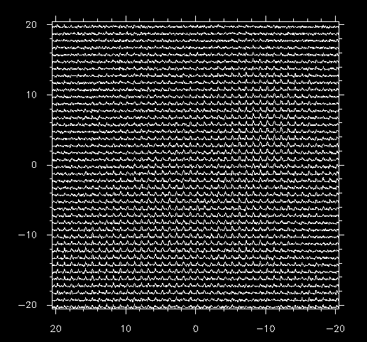
   LAS> set mode x -4 9
   LAS> set mode y -2 10
   LAS> map
Here's what the resulting image looks like for our 20'x20' map. Although tightly crammed, the overall structure of the [CI] lines is apparent in this map. Clearly, we have good data to work with!
We are now interested in extracting important information from this data cube. Making moment maps of the data are perhaps the most illustrative method of representing data. The print moment command will extract this information:
LAS> print moment 0 6 /output moments.txt
The output of print moment looks like this:
        213    -10.000    -15.000   5.9763       5.6309       1.6945
        214     -9.000    -15.000   6.1831       5.1198       1.8751
        [etc...etc...etc...]
The columns are, observation number, X and Y offsets,
integrated intensity, centroid velocity, and
linewidth.
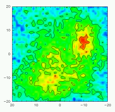
Now all that remains is to plot the results! We are done with CLASS; let's close it and open GREG. Let's also open up a color image plotting window, and set the plot to be square (since our map is the same size in RA and DEC):
   LAS> exit
   $ greg
   I-SIC,  Normal keyboard mode
   Default macro extension is .greg
   GreG> dev image white
   GreG> set box square
We will now utilize the column command to parse the various columns of the moments.txt file produced by print moemnt into X, Y, and Z arrays. X and Y are the RA and DEC offsets, and Z is the quantity we wish to plot. Let's first examine the integrated intensity (column 4).
GreG> column x 2 y 3 z 4 /file moments.txtNow, we'll load the column data into a regularly-spaced grid using rgdata, define the plotting limits from the data itself, resample the image to a 100x100 pixel image, draw everything to the plotting screen, redefine a better (AIPS-like) color palette, and then render a color Postscript file for printing:
    GreG> rgdata /blank 0
    GreG> limits /rgd
    GreG> resample 100 100 /blank 0
    GreG> box
    GreG> plot
    GreG> wedge
    GreG> let hue[i] = 256-2*i
    GreG> lut
    GreG> hardcopy plot.ps /dev ps color
And here's what the resulting image looks like on the screen:
 Basic processing Basic processing |
 Reduction Home Reduction Home |
 Processing OTF Maps Processing OTF Maps |