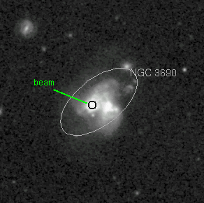
A digital sky survey image of the Arp 299 system of merging galaxies (also known as NGC 3690 or Markarian 171). The data we will analyze comes from the pointing labeled by the black circle.
Step 1: Loading CLASS and accessing your data file
Let's explore data collected towards an extragalactic source, as this data reduction is relatively straight-forward. In particular, we will investigate 12CO J=3-2 emission from the Arp 299 system of merging galaxies, located 42 Mpc distant (140 million light years). First, let's load CLASS:
    $ cd data
    $ class
    I-SIC,  Normal keyboard mode
    Default macro extension is .class
    LAS>
The LAS prompt tells us that CLASS is ready to accept our
commands. First, let's load a data file using the file in
command, find all observations in the file using find and
listing them to the screen with list:
    LAS> file in april2001.smt
    I-CONVERT,  File is  [VAX to IEEE]
    I-INPUT,  apr2001-1.smt successfully opened
    LAS> find
    I-FIND,  8309 observations found
    LAS> list
  8307;  1 ZETAOPH      CO(3-2)      SMT-10M-B71      0.0       0.0   Eq  2036
  8308;  1 ZETAOPH      CO(3-2)      SMT-10M-B72      0.0       0.0   Eq  2036
  8309;  1 ZETAOPH      CO(3-2)      SMT-10M-B73      0.0       0.0   Eq  2036
  [....etc...etc....etc....]
    LAS>
So far so good. The data file contains 8309 observations (including
calibration data). The list results provide a tabulation of
CLASS observation number, object name, name of spectral
line, name of telescope and spectrometer, angular
offsets in RA and DEC, and telescope observation number,
respectively.
Step 2: Extracting Relevant Spectra
As you can see, a CHEF-processed data file typically consists of a night (or an entire run) of data, so the first task is filtering the (potentially) thousands of spectra in the file to yield only the ones we are interested in. There are a number of methods of filtering that one will typically employ:
First, let's set the spectral line to CO(3-2), the object to ARP299A, and the spectrometer to the 1 MHz AOS (named SMT-10M-B30):
    LAS> set source arp299a
    LAS> set line co(3-2)
    LAS> set tel smt-10m-b30
    LAS> find
   I-FIND,  14 observations found
    LAS> list
I-LISTE,  Current index :
    49;  1 ARP299A      CO(3-2)      SMT-10M-B30      0.0       0.0   Eq  1828
    51;  1 ARP299A      CO(3-2)      SMT-10M-B30      0.0       0.0   Eq  1829
    59;  1 ARP299A      CO(3-2)      SMT-10M-B30      0.0       0.0   Eq  1832
    67;  1 ARP299A      CO(3-2)      SMT-10M-B30      0.0       0.0   Eq  1835
    75;  1 ARP299A      CO(3-2)      SMT-10M-B30      0.0       0.0   Eq  1838
    83;  1 ARP299A      CO(3-2)      SMT-10M-B30      0.0       0.0   Eq  1841
    85;  1 ARP299A      CO(3-2)      SMT-10M-B30      0.0       0.0   Eq  1842
  8181;  1 ARP299A      CO(3-2)      SMT-10M-B30      0.0       0.0   Eq  2004
  8189;  1 ARP299A      CO(3-2)      SMT-10M-B30      0.0       0.0   Eq  2007
  8197;  1 ARP299A      CO(3-2)      SMT-10M-B30    -21.000    -6.000 Eq  2010
  8205;  1 ARP299A      CO(3-2)      SMT-10M-B30    -21.000    -6.000 Eq  2013
  8211;  1 ARP299A      CO(3-2)      SMT-10M-B30    -21.000    -6.000 Eq  2016
  8219;  1 ARP299A      CO(3-2)      SMT-10M-B30    -23.000    +5.000 Eq  2019
  8227;  1 ARP299A      CO(3-2)      SMT-10M-B30    -23.000    +5.000 Eq  2022
    LAS>
Notice that our list of applicable observatiosn went from 8000 to only
14. Even now, notice that we took data at the on source (0,0)
position, as well as data at (-21",-6") and (-23",+5"). These data
correspond to other nuclei in the galaxy merger system; let's remove
them for now and concentrate on the (0,0) position:
    LAS> set offset 0 0
    LAS> find
    I-FIND,  9 observations found
    LAS> list
I-LISTE,  Current index :
    49;  1 ARP299A      CO(3-2)      SMT-10M-B30      0.0       0.0   Eq  1828
    51;  1 ARP299A      CO(3-2)      SMT-10M-B30      0.0       0.0   Eq  1829
    59;  1 ARP299A      CO(3-2)      SMT-10M-B30      0.0       0.0   Eq  1832
    67;  1 ARP299A      CO(3-2)      SMT-10M-B30      0.0       0.0   Eq  1835
    75;  1 ARP299A      CO(3-2)      SMT-10M-B30      0.0       0.0   Eq  1838
    83;  1 ARP299A      CO(3-2)      SMT-10M-B30      0.0       0.0   Eq  1841
    85;  1 ARP299A      CO(3-2)      SMT-10M-B30      0.0       0.0   Eq  1842
  8181;  1 ARP299A      CO(3-2)      SMT-10M-B30      0.0       0.0   Eq  2004
  8189;  1 ARP299A      CO(3-2)      SMT-10M-B30      0.0       0.0   Eq  2007
    LAS>
Good! Now we have data from two nights (notice the discontinuity in
observation numbers?) of the same object, same spectral line, same
offset in our list. Let's look at one of the spectra; first open up a
graphics window, get one of the spectra, and then type plot:
    LAS> dev xland black
I-X,  X-Window default version $Revision: 4.49 $ $Date: 1997/10/22 13:23:46 $
I-X,  Device DISPLAY :0.0
I-X,  Screen characteristics 16 planes, TrueColor
I-X,  Backing Store NOT supported
I-X,  Vendor The XFree86 Project, Inc; release 4003
I-X,  Protocol X11 ;revision: 0
I-X,  Screen size (mm) : height: 241, width: 333
I-X,  Screen pixels : height: 864, width: 1152
W-X,  B&W Window, dithering used for images
Graphics device /dev/tty successfully defined as a XLANDSCAPE BLACK
    LAS> get 51
    LAS> plot
Here is the resulting plot:
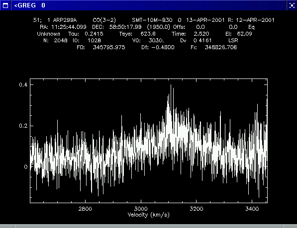
The header is plotted verbosely as well, which is enabled by typing set format long and disabled by set format brief. The important information labeled is:
Well, there might be something in the spectrum, but this is a scant 2 minutes of on-source integration time. We need to coadd the other frames:
    LAS> sum
I-GET,  Entry 49 Observation 49; 1 Scan 1828
I-GET,  Entry 51 Observation 51; 1 Scan 1829
I-GET,  Entry 59 Observation 59; 1 Scan 1832
I-GET,  Entry 67 Observation 67; 1 Scan 1835
I-GET,  Entry 75 Observation 75; 1 Scan 1838
I-GET,  Entry 83 Observation 83; 1 Scan 1841
I-GET,  Entry 85 Observation 85; 1 Scan 1842
I-GET,  Entry 8181 Observation 8181; 1 Scan 2004
I-GET,  Entry 8189 Observation 8189; 1 Scan 2007
   LAS> plot
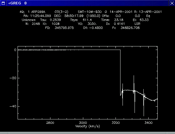
Uh oh. What happened? One of the contributing scans must be bad. Looking at a few of them, we see that observation 83 is bogus (and the logs show an AOS read error in that scan). Let's drop that observation from our list:
    LAS> drop 83
    LAS> list
I-LISTE,  Current index :
    49;  1 ARP299A      CO(3-2)      SMT-10M-B30      0.0       0.0   Eq  1828
    51;  1 ARP299A      CO(3-2)      SMT-10M-B30      0.0       0.0   Eq  1829
    59;  1 ARP299A      CO(3-2)      SMT-10M-B30      0.0       0.0   Eq  1832
    67;  1 ARP299A      CO(3-2)      SMT-10M-B30      0.0       0.0   Eq  1835
    75;  1 ARP299A      CO(3-2)      SMT-10M-B30      0.0       0.0   Eq  1838
    85;  1 ARP299A      CO(3-2)      SMT-10M-B30      0.0       0.0   Eq  1842
  8181;  1 ARP299A      CO(3-2)      SMT-10M-B30      0.0       0.0   Eq  2004
  8189;  1 ARP299A      CO(3-2)      SMT-10M-B30      0.0       0.0   Eq  2007
   LAS> sum
   LAS> plot
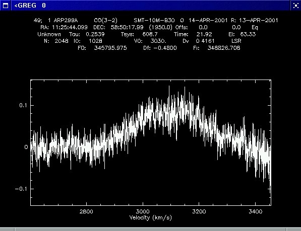
Since the line width is huge, our spectral resolution of 1 km/s is excessive. Let's smooth the spectrum to a coarser resolution with smooth. Each application of smooth halves the spectral resolution. We then will fit a Gaussian to the spectrum (gauss) and then show the fit on the screen (fit):
    LAS> smo
    LAS> smo
    LAS> smo
    LAS> plot
    LAS> gauss
 Guesses:   32.4         3.138E+03      278.
 SIMPLEX Minimization has converged
 RMS of Residuals :  Base =  1.00E-02  Line =  1.10E-02
 HESSE Second derivative matrix inverted
 MIGRAD Minimization has converged
 RMS of Residuals :  Base =  1.02E-02  Line =  1.10E-02

               FIT Results

 Line      Area               Position           Width              Intensity
  1   33.195     (  0.490) 3114.124 (  2.286)  313.235 (  5.254)  9.95556E-02
    LAS> fit
Here's the final spectrum:
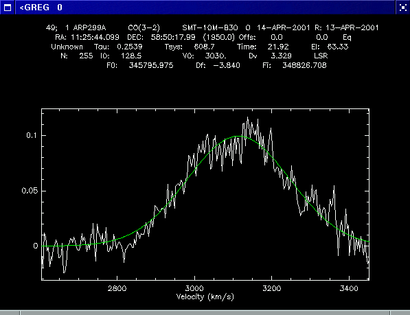
Cool! The data now has a 2-pixel resolution of 6.6 km/s. The data provided by gauss is very useful indeed; we see that the integrated intensity of our CO 3-2 line is 33.2 K km/s, centered at 3114 km/s VLSR, and has a linewidth (measured at half-maximum) of 313 km/s. Formal uncertainties are provided in parentheses. This yields an estimate of the H2 mass, redshift (and distance) to the galaxy, and kinematics of the gas in the galaxy.
An extremely simple-minded but illustrative analysis might look like the following:
Distance to Arp 299:
D(Mpc) = V/H0 = 3114/75 = 41.5 Mpc
Projected size of the 23" beam on the galaxy:
         D x theta(arcsec)
     S = ----------------
              206265

       = 41.5 Mpc * 23 arcsec
         --------------------
          206265

       = 4600 pc
Enclosed Dynamical Mass:
This involves all sorts of assumptions (virial equilibrium, centrally condensed mass distribution, speherical symmetry, the gas is accurately tracing the dynamical mass, etc...). Nevertheless, let's just see what happens:
       v2 * r
  M =  -----------
          G

    =  3132 (km/s)2 * 2300 pc
       ---------------------
       6.67*10-8

    =  (3.13*107 cm/s)2 * 6.9*1021 cm
       -------------------------------------
             6.67*10-8

    =  1044 g = 5*1010 Msun in the central 23"
Mass of H2:
The traditional method of estimating H2 mass stems from the linewidth-cloud size relation of Galactic Giant Molecular Clouds established in the 1980's. Assumptions: clouds are in virial equilibrium, gravitationally bound, same metallicity, temperature and density as Milky Way clouds. Thusly, there is good reason to believe that this conversion factor is NOT universal, so keep that in mind. Furthermore, we assume that the gas is warm, because we explicitly assume that the integrated intensity of the 3-2 line is similar to the 1-0 line. Nevertheless, with no other analysis, let's just see what we get:
N(H2) [cm-2] = 2*1020 * I(CO J=1-0) [K km/s]

                                   = 2*1020 * 33 K km/s
                                   = 6.6*1021 cm-2
This is the mean N(H2) over the whole beam. What is the
surface area of the beam? Assuming the beam is the projection of a
sphere:
    pi * beam-radius2 = 3.14159 * (6.9*1021 cm)2
                                 = 1.5*1044 cm2
So the number of H2 molecules is N(H2) * area:
                            = 6.6*1021 cm-2 * 1.5*1044 cm2
                            = 9.9*1065 molecules

                            = 9.9*1065 * 12*10-24g/molecule = 1.1*1043 g
                            = 6*109 Msun
About 10% of the dynamical mass. Vaguely sensible. :)
 Installing GILDAS Installing GILDAS |
 Reduction Home Reduction Home |
 Regularly Sampled Maps Regularly Sampled Maps |