Reduction of Randomly-Sampled On-The-Fly Maps

On-the-fly maps generate readouts of the spectrometers at typically fixed time intervals, rather than fixed positions on the sky. Slight acceleration or deceleration of the antenna makes for an irregularly-sampled map, although often only slightly. This map must be gridded and convolved before proper analysis can be performed upon it.
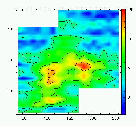
Let's look at a HCO+ J=4-3 (356 GHz) map of the rho Oph dark cloud, in the vicinity of the rho Oph A core. The data are sampled every 3 seconds, as the telescope moves 80 arcseconds per minute. Only one pass over the map is made. This leads to 1/6th beam sampling, which eliminates blurring in the scan direction. Faster scanning, up to 1/4th beam per sample, is also routinely performed at the HHT.
First, we perform basic processing as we did with the regularly sampled data (removal of low-order fits to the baseline). Opening the new processed file, we now utilize the grid command in CLASS to regrid and convolve the data to the beam size (which is 22" at 356 GHz), storing the channels between -20 and 30 km/s Vlsr to the data cube:
    LAS> file in hcop43.smt
    LAS> find
    I-FIND, 1503 observations found
    LAS> grid hcop43.gtf new /channel v -20 30 /image beam 22
I-GET,  Entry 1299 Observation 5976; 2 Scan 2262
I-GET,  Entry 1300 Observation 5979; 2 Scan 2262
I-GET,  Entry 1301 Observation 5982; 2 Scan 2262
[etc...etc...etc...]
I-GRID,  Beam size 22.00"
I-DOSOR,  Sorting input table
I-SUB_GRID,  Creating a cube with 21 by 31 pixels; pixel -11.0" x 11.0"
I-GRDFLT,  X Convolution Exponential Par.= 1.8000 0.3603 2.0000
I-GRDFLT,  Y Convolution Exponential Par.= 1.8000 0.3603 2.0000
I-SUB_GRID,  Creating map file test.lmv
I-SUB_GRID,  Updating map
    LAS>
Now we are done with CLASS. Let's move to GRAPHIC for the rest of the reduction process. We'll also open a color graphics window for plotting.
    $ graphic
I-SIC,  Normal keyboard mode
Default macro extension is .graphic
    GRAPHIC> dev image white
I-X,  X-Window default version $Revision: 4.49 $ $Date: 1997/10/22 13:23:46 $
I-X,  Device DISPLAY :0.0
I-X,  Screen characteristics 16 planes, TrueColor
I-X,  Backing Store NOT supported
I-X,  Vendor The XFree86 Project, Inc; release 4003
I-X,  Protocol X11 ;revision: 0
I-X,  Screen size (mm) : height: 241, width: 333
I-X,  Screen pixels : height: 864, width: 1152
Graphics device /dev/tty successfully defined as a IMAGE WHITE
    GRAPHIC>
So far, this looks uncannily like CLASS. Most GILDAS programs act
fundamentally the same way, for better or worse. Now we will run a
GILDAS task called 'moments'. It performs a similar task to the
'print' command (see regularly sampled
maps), for inhomogenously-sampled data gridded by CLASS and stored
in a GTF or LMV file.
   GRAPHIC> run moments
Input file name
FILE        IN$                              = hcop43.lmv
Output files name (no extension)
FILE        OUT$                             = hcop43
Velocity range
REAL        VELOCITY$[2]                     = 0 6
Detection threshold
REAL        THRESHOLD$                       = 0
Smooth before detetction ?
LOGICAL     SMOOTH$                          = no
I-RUN,  Task moments running, logfile is
        /home/ckulesa/moments.gildas
We have asked it to take the LMV file created by CLASS's grid
command and create the first three moment maps for us, given that the
line window is between 0 and 6 km/s Vlsr. Moments has written three files: hcop43.mean, an image containing the integrated
intensities; hcop43.velo, an image containing the centroid
velocities; and hcop43.width, an image containing the line width
map.
Let's plot the integrated intensity, take the X-Y-intensity plotting limits from the actual data, plot a color wedge, resample to a 100x100 pixel image, and set an AIPS-like color scheme, set contour spacing to 4 K km/s (starting at 4 K km/s), plot the contours, and generate a color Postscript file for printing:
    GRAPHIC> image hcop43.mean
W-GDF_RHSEC,  Absent section EXTREMA
W-GDF_RHSEC,  Absent section RESOLUTION
W-GDF_RHSEC,  Absent section NOISE
    GRAPHIC> limits /rgd
    GRAPHIC> set box square
    GRAPHIC> plot
    GRAPHIC> wedge
    GRAPHIC> resample 100 100 /bl 0
I-RESAMPLE,  Got    79 pages of virtual memory
    GRAPHIC> box /u s
S-CHAR,  Fonts loaded
    GRAPHIC> let hue[i] = 256-2*i
    GRAPHIC> lut
    GRAPHIC> plot
    GRAPHIC> wed
    GRAPHIC> levels 4 to 30 by 4
I-LEVELS,  Contour levels are :
     4.000         8.000         12.00         16.00         20.00
     24.00         28.00
    GRAPHIC> rgmap
I-RGMAP,  Contouring checks the blanking value   0.00000
I-RGMAP,  Pens  0 & 15 used for positive & negative levels
I-RGMAP,  Contour   1   4.00000
I-RGMAP,  Contour   2   8.00000
I-RGMAP,  Contour   3   12.0000
I-RGMAP,  Contour   4   16.0000
I-RGMAP,  Contour   5   20.0000
I-RGMAP,  Contour   6   24.0000
I-RGMAP,  Contour   7   28.0000
    GRAPHIC> hardcopy hcop43.ps /dev ps color
And here is what it looks like:
 Regularly Sampled Maps Regularly Sampled Maps |
 Reduction Home Reduction Home |
 Making Fancy Plots Making Fancy Plots |