Removal of Atmospheric Features

The first step is to process your comparison star's spectrum in precisely the same way you processed your object spectrum. Once you have an extracted comparison star spectrum of high S/N, you can divide it into your object spectrum. In principle, you could do this with plain old imarith, like this:

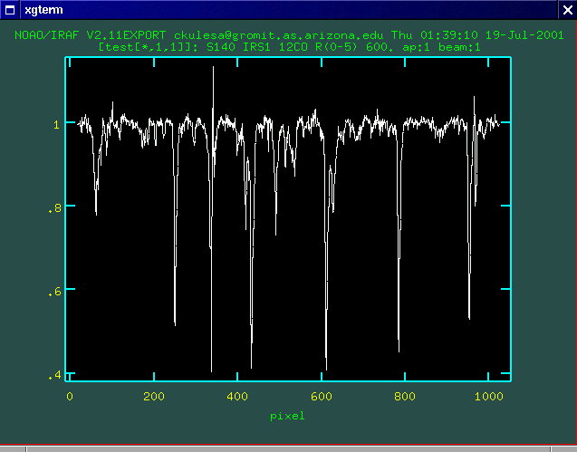
imarith s140_4272.ms / brightstar s140_4272-done

Here's what you get if you do this... it's certainly cleaned up to an extent, but it's far from pretty.

Unfortunately, the real world plays nasty tricks on poor astronomers, and a lot of tweaking is needed to remove telluric features. This makes using imarith painful, to put it mildly.

• For one, the atmosphere might change faster than the elapsed time between the acquisition of your object and comparison star data. One way around this is to interleave observations of comparison stars with your program scientific targets. Bad news: this increases overhead on objects that are not visible on the optical guider because an object must be re-acquired on the slit of Phoenix.
• Another issue is that the comparison star is looking through a different airmass than the science target. This can be minimized by careful selection of comparison stars. Bad news: there aren't many bright, hot stars at 3-5 microns, so the pickins' are slim.
• The Phoenix grating has a tendency to creep slightly in the first hour or so after it is set. Even if you carefully align all frames spectrally before combination, it is very possible that your scientific target and comparison star spectra will be slightly skewed, perhaps up to 2 km/s, or a little over 1 pixel.

What we need to do is scale the comparison spectrum (ala Beer's Law) to match the depth of the atmospheric features in the object spectrum. Additionally, we need to be able to shift the comparison spectrum in wavelength to allow maximum cancellation of features. Even a shift of 0.1 pixel is enough to obliterate weak spectral features in the vicinity of saturated atmospheric features.

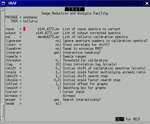
Fortunately, there is an alternative to painful iterative use of imarith. The telluric task provides an interactive, graphical way to iteratively yield excellent cancellation of atmospheric features. The interface is a bit clunky and confusing at first, but once you get the hang of it, it's not so bad.

Click here for text parameters

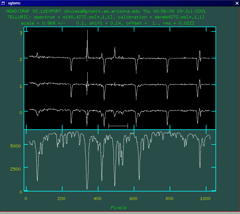
The comparison spectrum is shown in gray in the bottom-most panel (you can choose to toggle with the object spectrum, see table below).

The stacked display shows three corrected candidate spectra. The center one is for the current shift and scale and the other two are one step higher or lower in the shift or scale. The current values and the step is shown in the title. Toggle between the shift and scale modes with x or y. Once a mode is selected, select the best spectrum with the cursor and type x or y to make it the current (middle) spectrum.

In this case, the top spectrum grossly over-corrects for telluric features. The bottom one grossly under-corrects. The middle one isn't too bad. But clearly, the steps between the three spectra are too coarse. To fine-tune either the shift or scale, select the middle spectrum and hit x or y, respectively. That will reduce the step by a factor of two. If you want to increase the step size, select x or y on the middle spectrum and then hit e.

As usual, q quits the task, and the middle spectrum is saved.

That sounds complicated in words... so here's a summary table:

Keystroke	Result
x	Switches to shift mode, if in scale mode. Once in shift mode, hitting x on the middle spectrum will decrease the step size. Hitting x on the upper or lower spectrum will make it the new current spectrum.
y	Switches to scale mode, if in shift mode. Once in scale mode, hitting y on the middle spectrum will decrease the step size. Hitting y on the upper or lower spectrum will make it the new current spectrum.
e	When in either shift or scale mode, increases the step size.
d	Toggles the data spectrum in the bottom panel
c	Toggles the comparison spectrum in the bottom panel
s	Use this key to mark the extent of a sample region for statistics. You can use the computed RMS of this region as a numerical figure of merit as you interactively try to minimize the telluric features. Or use it with the automatic RMS minimization feature, below.
a	Automatically pick the best scale and/or shift to minimize the RMS residuals in the defined sample region, above.
?	Online help
q	Quits, and saves the middle spectrum.

Whew! Now let's have a look at our spectrum using splot. We can normalize our spectrum, removing any residual continuum shape. In splot, type t to select a continuum-fitting routine. Select / for continuum normalization (versus, say, continuum subtraction), and then select the appropriate order of fit (ex. :o 9) and refit (f) until it looks sensible. Then hit q. You can save the new spectrum by hitting i and providing a filename.

Here's the corrected spectrum, with a 5% scaling of the comparison spectrum and a shift of 0.2 pixels (0.3 km/s).

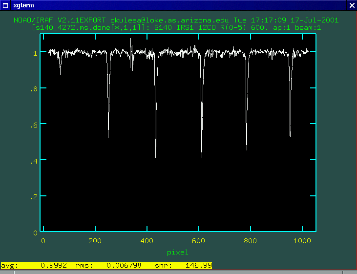
Our final spectrum has an average S/N of about 150. Not too shabby for a 1-arcsecond slit, guiding by the "seat of our pants" (no optically-visible targets) for about 80 minutes on the old noisy Aladdin I array! We could actually do science with this spectrum now, but we'd like to apply a wavelength calibration first. On to the last step!

Extracting a 1D Spectrum

Reduction Home

Wavenumber Calibration